As part of our guest blog series, we bring you a post from Kathryn Shafer. A former middle school and high school math teacher, Kathy is now an Assistant Professor in the Department of Mathematical Sciences at Ball State University, Indiana. She’s done a variety of work for Key, including presenting webinars, moderating online courses, and delivering face-to-face professional development workshops.This summer, the teachers in my probability and statistics course used TinkerPlots to complete an exercise on the Law of Large Numbers. An engaging discussion took place, as a few of the teachers wanted to discuss their interpretations of graphs, and others extended the problem beyond what was required. The resulting discussion focused on simulation models and multiple representations, hitting the mark with regard to the  Mathematical Practices.

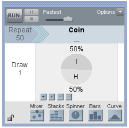
A coin flip experiment can be modeled used the Sampler Engine in TinkerPlots. Set the Sampler options to capture the running percent of heads. The Spinner device can be used to simulate a fair coin. The spinner shown at right will simulate flipping a fair coin 50 times.

As one of the teachers discussed the running percent calculation, I suggested we add the attribute “running count of heads” to the Case Table. The teacher used this to explain that the ratio of the number of heads to the number of trials will produce the running percent.

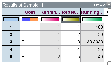
She then explained how these values match the coordinates of the first three points in the scatterplot shown below: (1, 100), (2, 50) and (3, 33.3). After 50 trials, the percent is bouncing above 50%. It will take a lot more trials to settle down close to 50%.

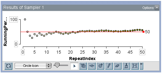
Another teacher offered an approach she planned to use with her fifth graders. Her idea was to begin with a small number of trials and notice what changes at say, 10 flips, 50 flips and then 100 flips. This supports how middle grade students think about probability, through an investigation of individual cases or data points.

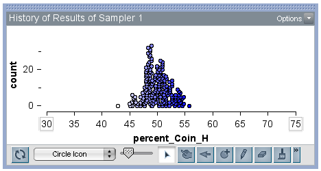
Next, a teacher showed how he used the History tool to capture and graph 288 samples of 500 coin flips. His comment was, “Is this the Normal Distribution? It sure looks like it.” We launched into a discussion of the properties of the Binomial Distribution and how the graph of the percent heads will have the properties of the Normal Distribution (given that certain conditions are met). The graph shown below was created with 200 samples of 50 trials. The teacher had used the Standard Deviation Hat Plot and the Drawing tool to justify his claim that this was a Normal Distribution.

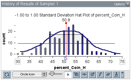
A follow-up question that could have been asked is, “What would happen if we increase the number of trials in each sample?” In the graph below, I changed the Repeat number to 500, cleared the History case table, and collected 200 samples of the running percentages of heads. We see how the variability drastically decreased from a range of approximately 45% to a range of about 10%.

To wrap up the discussion of the Law of Large Numbers, we designed a quiz problem. This involved a Spinner set to two unequal sectors that were hidden and locked with a password. The teachers were challenged to decide if the coin was fair and if not, to make a conjecture as to how it was weighted.

The use of TinkerPlots allowed the teachers to quickly explore the “what if” types of questions that arise in the context of probability, modeling the type of exploration I hope teachers will use with their students in the classroom.