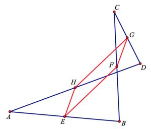
In the interactive Web Sketchpad model below (and here on its own page), ABCD is an arbitrary quadrilateral whose midpoints form quadrilateral EFGH. Drag any vertex of ABCD. What do you notice about EFGH?

The midpoint quadrilateral theorem, attributed to the French mathematician Pierre Varignon, is relatively new in the canon of geometry theorems, dating to 1731. Mathematics educator Chris Pritchard says the theorem “epitomises simplicity, economy, and elegance….And even today, in an idle moment, I find myself doodling…perhaps still seeking a quadrilateral for which Varignon’s theorem doesn’t hold.”

Varignon theorem is also a poster child for the benefits of dynamic geometry software, appearing regularly in articles that introduce readers to the pedagogical opportunities afforded by the software. Below are four commonly cited ways in which  Varignon’s theorem illuminates the power of dynamic geometry:

1. 1. The theorem is dramatic and unexpected: Who would believe that a random quadrilateral ABCD  has the DNA of a parallelogram within it, ready to be uncovered by connecting its midpoints? Dynamic geometry amplifies the discovery and the ‘wow’ factor, showing not just one parallelogram but an entire collection of them as you drag the construction.
   2. The theorem nicely illustrates the ability of dynamic geometry software to explore  “monster” cases that normally do not receive attention. Using the software, you can drag a vertex of ABCD so that the quadrilateral becomes pretzel-like in appearance and still EFGH is a parallelogram.
   3.  The theorem demonstrates the role of dynamic geometry in establishing our conviction that EFGH is a parallelogram. Had you viewed a single static image of the construction, you would have little reason to believe that EFGH was always a parallelogram. But the data you obtain from dragging the construction leaves little doubt about what you’re observing. With this firm belief about EFGH’s properties in place, proof becomes a vehicle not for assuaging our doubts but rather for helping you to  understand why the quadrilateral is a parallelogram.
   4. The proof of the theorem can be scaffolded with the help of the software. Ask students to construct  the two diagonals AC and BD of ABCD and see what they observe and can figure out. Students might measure the lengths of AC, EF, and GH, and then drag the construction, noticing that AC is always twice the length of EF and GH. The combination of the diagonal and the measurements helps them to recognize the triangle midsegment theorem applied to ΔABC and ΔADC.

I think items 1–3 above showcase dynamic geometry at its best, but I’m less enthusiastic about dynamic geometry software’s role in the proof of Varignon’s theorem in item 4. Telling students to construct the diagonals of the parallelogram feels like we’re depriving them of the aha! moment of realizing that the proof is nothing more than several applications of the triangle midsegment theorem. Below are  two ways that we might make better use of dynamic geometry to motivate a proof of Varignon’s theorem. Each focuses on a degenerate case of the construction, turning quadrilateral ABCD into a triangle.

Ask students to drag a vertex of ABCD so that two sides of the parallelogram overlap

While exploring this task, students discover that the overlapping occurs when two opposite vertices of ABCD coincide (points B and D in the picture below). In fact, not only do the sides of the presumed parallelogram overlap, but its remaining two sides disappear entirely. The image below is certainly suggestive of the triangle midsegment theorem—it’s only missing segment AC. To gather more visual data, students can drag point C to view a collection of triangles ADC (with missing side AC), all displaying their midsegment.

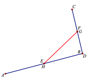
Ask students to drag a vertex of ABCD so that the vertex is collinear with its two adjacent vertices

The picture below shows one such location of point B. By construction, EB is always half the length of AB and FB is always half the length of CB regardless of point B’s location. Segment EF, which is composed of EB and FB, is thus half the length of AC. If we assume, based on our observations of dragging point B, that GH is equal to EF, then GH is equal to half the length AC. This statement rings a bell—it’s the triangle midsegment theorem. By assuming that EF = GH, we’ve found a result that helps us to backtrack and explain why the two lengths are equal.

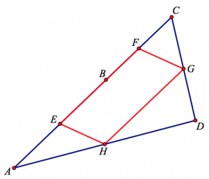
And as a bonus, the picture below suggests another theorem: Start with a triangle ACD and construct midpoints G and H on two of its sides. On the third side, AC, construct midpoint B and then construct midpoints E and F of AB and CB, respectively. Connect points E, F, G, and H. They form a parallelogram. You can view this model on the second page of the websketch at the top of the page by clicking the arrow in its lower-right corner.

Varignon’s Converse

Finally, the Web Sketchpad model below (and here on its own page) shows a fascinating variation of Varignon’s theorem described by Celia Hoyles in The Changing Shape of Geometry. We start with a random quadrilateral ABCD and a point E. Construct a segment EF passing through vertex B so that EB = BF.  Then construct FG, passing through vertex C, so that FC = CG. Continue this construction method with GH and HI. Now, drag point E. Notice that vector IE maintains its length and direction. Can you prove why?

Hoyles writes, “…when I noticed the invariant vector and could explain it, my perspective on the original theorem completely changed. I now see Varignon as a particular case of a more general theorem, which can be stated informally as follows: every quadrilateral has associated with it a fixed vector IE, which just happens to be zero when the original quadrilateral is a parallelogram.”